Lesson 3 - Jupyter Notebook

Introduction

Aim of the class

At the end of this class, you will be able to:

• Create your own environment to run your Jupyter Notebook
• Create, run, export your own Jupyter Notebook
• Know about magic commands
• Use interactivity with a Jupyter Notebook

This last class is also to keep on praticing the notions learned in the previous lessons.

Jupyter Notebook

What is Jupyter Notebook

A Jupyter Notebook is a computational notebook with the file extension .ipynb. It is a document that can combines text (formatted in plain text or Markdown), code (python, R, bash) and various visualizations (such as graphs, tables). It provides a friendly environment to format, explain and explore the results of a data analysis. Jupyter Notebooks can be exported to .pdf or .html to share them easily.

It is part of the Project Jupyter, which is an umbrella project providing tools for interactive computing. JupyterLab provides an environment and user interface for Jupyter Notebooks.

How can I program in a Jupyter Notebook

In your text editor

To use Jupyter Notebook outside of a JupyterLab, your text editor must be compatible with the Jupyter Notebook format. In Visual Studio Code, you will need to install the Jupyter extension. Some other extensions can be useful, for example Jupyter Cell Tags.

On a local server

If Jupyter Notebook or Jupyter Lab is installed (report to installation doc) on your computer, you can start running a local notebook server by running in the terminal:

jupyter notebook 

or

jupyter lab 

This will print some information about the notebook server in your console, and open a web browser to the URL of the local web application.

Inside a JupyterLab

In the IGBMC, you can for example have access to a JupyterLab on the cluster with Open OnDemand.

For test purpose, you can also create a Jupyter Notebook in JupyterLab.

Conda environment as a kernel

A Kernel is a computational engine for running and interacting with the Jupyter code. By default, Jupyter only knows about the base Python environment. This Python environment needs to have the necessary python library installed (e.g. pandas, matplotlib).

In some cases, it might be useful to create different Python environments for different usage or projects. This ensures that you can install specific packages and Python versions without affecting your base system or other environments. For this purpose, a common tool used is conda.

Figure 6.1: Conda schema from https://angus.readthedocs.io/

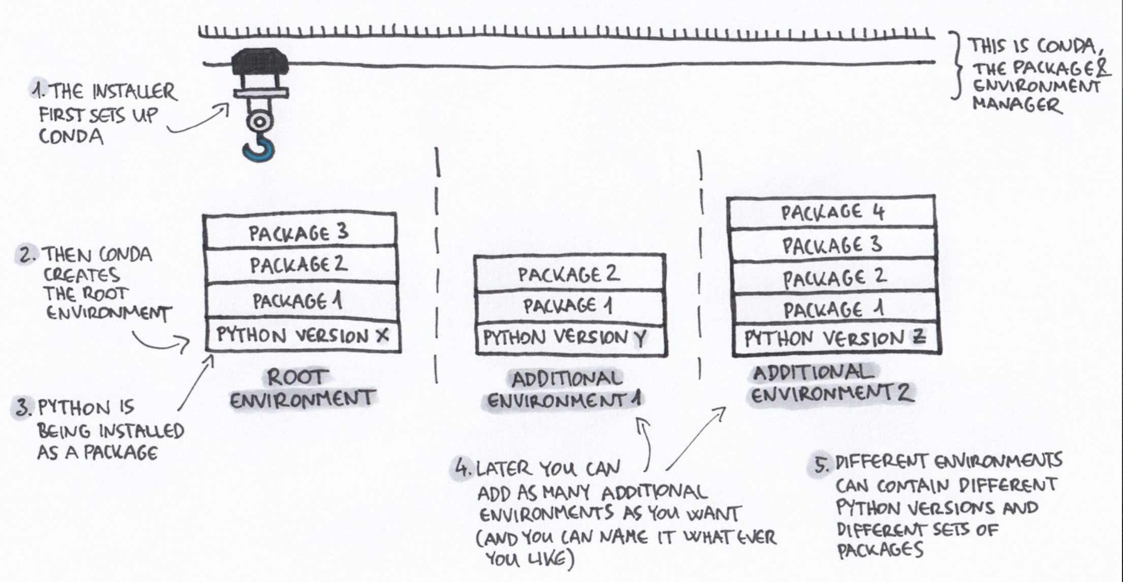
You can see it as a closed setup with its own Python interpreter and packages.

Some basic library like pandas or matplotlib are included in most already existing Kernels. But other library that are domain-specific won’t be included by default. Also, you might want to work with a specific version of python or python packages.
It is possible to register a Conda environment as a Kernel (so that Jupyter can use an environment with adequate packages to run code).

# Run just once after installing conda, to actually start working in conda-mode
conda init 

# Open a new terminal (for conda init to be effective)
conda create -n python_intro python
conda activate python_intro
conda install ipykernel notebook

# In some JupyterLab instances you need to run the following:
python -m ipykernel install --user --name=python_intro 

Exercise

Create the conda environment like above. The environment should now be available as a Kernel in the selection.

Run the command print('Hello World!') in a cell.

Run the command import pandas in a cell. If it does not work run in the terminal conda install pandas or pip install pandas, and once it’s installed, try re-running the command import pandas.

As we are using conda, we might as well get familiar with some basic commands in conda.

Command	Description
conda create -n env_name	Create a new environment
conda create -n env_name package	Create a new environment with a specific package
conda create -n env_name package==version	Create a new environment with a specific package and version
conda activate env_name	Activate an environment
conda deactivate	Deactivate the current environment
conda list	List all installed packages in the current env
conda env list	List all available environments
conda install package_name	Install a package in the current environment
conda remove package_name	Remove a package from the current environment
conda remove -n env_name --all	Remove an entire environment
conda update package_name	Update a specific package
conda update conda	Update conda itself
conda search package_name	Search for a package in conda repositories
conda info	Display information about the conda installation

Exercise

Try the commands conda list and conda env list. Do you understand what they output?

Create an environment with pandas at version 1.5.3. You can verify the version of pandas with the following python code print(pandas.__version__).

Solutions

conda list prints the packages available in the current environment.

conda env list prints the conda environments available.

In a terminal run:

conda create -n pandas_v1 pandas==1.5.3
conda activate pandas==1.5.3
python -c "import pandas; print(pandas.__version__)"

Structure of a Jupyter Notebook

Cells

In practice, a notebook consists of cells. A cell can contain Markdown or code. The execution of a code cell is dependent on the kernel used (for example, the kernel needs to have the adequate python packages installed). The results and warnings returned are displayed as the cell’s output. The output can be text, table, plot…

Exercise

Let’s create our first Jupyter Notebook. For this create a new file and name it lesson-3-companion.ipynb. Before creating your Jupyter Notebook, (or before running your first cell) you will get asked to choose a Kernel. For the moment let’s use the first one provided, we’ll explain later what it is.

Write a command in the first cells that says print("Hello Jupyter") and execute it.

Write a command that will generate an error, for example print("Hello Jupyter", end=1) and execute it.

Solutions

See associated Jupyter Notebook or its html

Markdown

The aim of a Jupyter Notebook is also to explain code. For this, we can write in the Markdown format descriptions of the experiment, the dataset, or general useful information about the analysis.

In markdown, you can:

Create headers (i.e. titles with hierarchy):

# Header 1
# Header 2
## Subheader 1

Write in italics: *italics*

Write in bold: **bold**

Write links: [links](https://igbmc.fr)

Add images : ![alt text](img/jupyter.png){width=10%}

Create (nested) lists:

• Item 1
• Item 2
  • Subitem 1

- Item 1
- Item 2
  - Subitem 1

Write in html:

This is in red.

<p style="color:red;">This is in red.</p>

Exercise

Let’s rewrite some code of Exercise 3 of lesson 2 below into a Jupyter Notebook, with some explanation of the dataset and the code, using Markdown formatting.

Use at least the following Markdown elements:

• header
• bold
• list
• link

And execute at least the following code (seperate it in different cells).

import pandas as pd

df = pd.read_csv('exercise/data/example.txt', index_col=0, sep=' ')
df = pd.melt(df, var_name='nucl', value_name='freq', ignore_index=False)

df.index
df.columns

df.head()

df['freq'].mean()
df.groupby("nucl")[['freq']].mean()

Solutions

See associated Jupyter Notebook or its html

Magic Commands

Magic commands are handy commands built into the IPython kernel. You can get an explanation of all magic commands and usages in the IPython doc. Here are a few that can be useful:

Command	Usage
whos	Show a table of all vairables defined within the current notebook
history	Display command history
time	Measure execution time a Python statement or expression (line or cell)
writefile	Write the content of a cell into a file
load	Load content of an external python script into a cell
run	Execute an external python script
pip	Run the pip package manager within the current kernel

To use it in line mode add the prefix % before the command (e.g. %time). To use it in cell mode add the prefix %% (e.g. %%time). Some commands can only be used in one or the other mode.

Exercise

1. Load the file analyse_fasta.py that contains the functions nucl_freq() and analyse_fasta() into the next cell. Run the command nucl_freq("AACTTG") to verify that it worked.

2. Use a magic command to get all the variables currently defined. Remove the functions nucl_freq and analyse_fasta variable using del <variable> in python and rerun the magic command to output all variables currently defined.

3. Run the file analyse_fasta.py that contains the functions nucl_freq() and analyse_fasta(). Run the command nucl_freq("AACTTG") to verify that it worked.

Solutions

See associated Jupyter Notebook or its html

Exporting notebook

JupyterLab allows you to export your jupyter notebook files (.ipynb) into other file formats such as:

• HTML .html
• LaTeX .tex
• Markdown .md
• PDF .pdf
• Executable Script .py

Converting the notebook uses the module nbconvert and the availability of certain conversions will depend on nbconvert configuration.

On a JupterLab instance, you will be able to export your notebook with File > Save and Export Notebook As.

In the Visual Studio Code, exporting can be done with the button (on the same bar as + Code) ... > Export or via the Command Palette >Jupyter: Export to ....

Exercise

Export lesson-3-companion.ipynb in a .html format. Open the .html file into a browser.

Interactive notebook

Widgets

An interesting thing about notebook is to make them interactive. For this we will use the interact function of ipywidgets.

It can take different values as input (integer, boolean, string):

from ipywidgets import interact

def f(x):
    return x

interact(f, x=10)

interact(f, x=True)

interact(f, x='Hi there!')

interact(f, x=['Choice A', 'Choice B'])

Or more than one value:

def f(w, x, y, z,):
    return (w, x, y, z)

interact(f, w=10, x=True, y='Hi there!', z=['Choice A', 'Choice B'])

The type of value given calls for a specific widget (slider, check box, text box), that can be parametered. Here is a summary:

Type of value	Widget function	Usage example
Boolean	Checkbox()	True or False
String	Text()	'Hi there'
Integer	IntSlider()	value or (min,max) or (min,max,step) if integers are passed
Float	FloatSlider()	value or (min,max) or (min,max,step) if floats are passed
List	Dropdown()	['orange','apple'] or [('one', 1), ('two', 2)]

There are actually many more widgets, they can be found in ipywidget documentation.

Warning

The interactivity is only kept in the Jupyter Notebook format .ipynb as it needs the Kernel to be run. That means that these interactive elements will not be exported in the .html format for example.

Which is also why the exmaples given in this website are not interactive!

Exercise

Create an interactive plot based on the stacked bar chart from lesson 2. It should show the frequencies of only one (interactively) selected nucleotide for each sequence.

Export it in .html.

Bonus: allow for the choice of multiple nucleotides.

<function __main__.interactive_plot(columns)>

Solutions

import pandas as pd
import matplotlib.pyplot as plt
from ipywidgets import interact
from ipywidgets import widgets

# Create a DataFrame from the given data
df = pd.read_csv('exercise/data/example.txt', index_col=0, sep=' ')

def interactive_plot(columns):
    # Plot the data
    fig, ax = plt.subplots(1, figsize=(5, 6))

    bottom = pd.Series([0,0,0,0,0], index = df.index) 
    for col in columns:
        ax.bar(df.index, df[col], label=col, bottom=bottom)
        bottom += df[col]

    # Add labels and legend
    ax.set_xlabel('Sequences')
    ax.set_ylabel('Frequency')
    ax.legend(title='Nucleotides', bbox_to_anchor=(0, 1),
              loc='lower left', ncols=4)
    plt.show()

interact(interactive_plot, columns=df.columns)

interact(interactive_plot, columns=widgets.SelectMultiple(
    options=df.columns,
    value=[df.columns[0], df.columns[1]],
    description='Nucleotides',
    disabled=False
))

See associated Jupyter Notebook or its html

Plotly express

plotly.express is a module used to create figures that are interactive. Refer to its documentation for more information.

Warning

It does not rely on the same grammar as matplotlib, so you have to get used to new objects and functions to create plots. We will not cover it here, but it is useful to know that plotly.express exists when creating Jupyter Notebooks

import plotly.express as px
import pandas as pd

df = pd.read_csv('exercise/data/example.txt', sep=' ')
df = pd.melt(df, var_name='nucl', value_name='freq', id_vars=['Seq'])

fig = px.bar(df, x="Seq", y="freq", color = "nucl", title="Nucleotide frequency")
fig.show()

Final exercise

Exercise

Download the GSE165691_DEG_result_table.xlsx file from GEO.

Create a new Jupyter Notebook to analyze this dataset. Use markdown cells as necessary to explain the process and results of the analysis. Throughout the notebook, use the following markdown elements:

• header
• bold
• links
• lists

1. Load the dataset into the Notebook using pandas.

Hint

Run the magic command %pip install openpyxl inside a cell of the Notebook. Now you can use pd.read_excel()!

2. Explore the datatable and describe it (number of rows, columns, column names and what they contain…). Importantly, get the following information:

• are there any value that are null? If so in which columns?
• number of unique genes
• min, max and mean of log2FC
• number genes with of padj < 0.05
• number of significantly up- and down-regulated genes (up: log2FC > 1 and padj < 0.05 and down: log2FC < -1 and padj < 0.05)

Hint

For the last two information, you can make good use of either .sum() or .value_counts().

3. Get the following values:

• the expression in both samples of the genes: Il31ra, Sox9, Lbp
• the gene with the highest log2FoldChange, and the gene with the lowest log2FoldChange.

Hint

For the last one, you can use .idxmin(), see doc

4. Make a histogram plot of the log2FoldChange.

Hint

pandas has built-in plot functions that are based on matplotlib.

5. Make a pie plot that gives the proportion of positive-log2FoldChange genes and negative-log2FoldChange genes.

Hint

Compute the number of positive and negative log2FoldChange first. Then use plt.pie().

6. Make a volcano plot where up-regulated genes are red points, down-regulated genes are blue points, and other are grey.

Hint

Create a new column called color that has the value red for up-regulated genes, blue for down-regulated genes, and grey for others.

7. Just like 6 but make it interactive with widgets so that you can change the threshold of log2FoldChange and padj.

8. Just like 6 but make it interactive with plotly expression so that you can hoover your mouse on a point and get the name of the gene, and some other informations available about that gene (e.g. 'ensembl_gene_id', 'log2FoldChange', 'padj', 'symbol','PR661W_Vec', 'PR661W_TRPM1').

Hint

plotly.express behaves differently than matplotlib. You can create a new column called color that has the value up-regulated for up-regulated genes, down-regulated for down-regulated genes, and Non-significant for others.

9. Make a heatmap of the top 5 up-regulated and top 5 down-regulated (based on log2FoldChange) genes where the color corresponds to the log value of norm.count.mean column.

Hint

One way to order by absolute value of a column is: df.sort_values(..., key=lambda x: abs(x)).

Use np.log() from numpy package.

10. Export the notebook in html.

Solutions

See associated Jupyter Notebook or its html

References

Here are some references and ressources that inspired this class:

• Jupyter doc
• NIG course